Concepts
Data Reduction
HiDRA utilizes an Experimental Physics and Industrial Control System (EPICS) based control software with the neutron Event Distributor (nED) data acquisition system. 13,14 See ref 15 for additional details about the EPICS base framework. HiDRA measures neutrons using a DYNEX He3 2D position-sensitive detector with a 30x30 cm2 active detection area. The nED system records measured neutrons into an event-based nexus file with information about both the pixel position and detection time, which provides a time-stamp of the total time elapsed from the start of the measurement to the detection of each neutron event. HiDRA utilizes the event data structure to store common measurements, e.g., pole figures or strain maps, in a single raw neutron event nexus file with “sub-runs” defined by incrementing a sub-run flag. pyRS uses these timestamps and sub-run flags to reduce neutron event data into N I(Px, Py) data arrays, where N is the number of sub-runs within a file.

Converting raw neutron events from I(Px, Py) into I(2θ) requires accurate knowledge of the detector in space. The detector shield box at HiDRA is positioned on a 2θ arm that is equipped with a precision Heidenhain encoder, which provides an accurate and precise reference point (0.003° 2θ reproducibility). A detector calibration routine was established to determine the relative shifts and tilts of the detector with respect to the 2θ arm.
Powder Reduction
pyRS integrates measured 2D into 1D data based on the (x, y, z) coordinates of each pixel. The position of each pixel is determined based on the angular position of the detector (2θ) and calibrated detector shifts and rotations. The pixel positions are converted in to angular (2θ, η) maps using
and
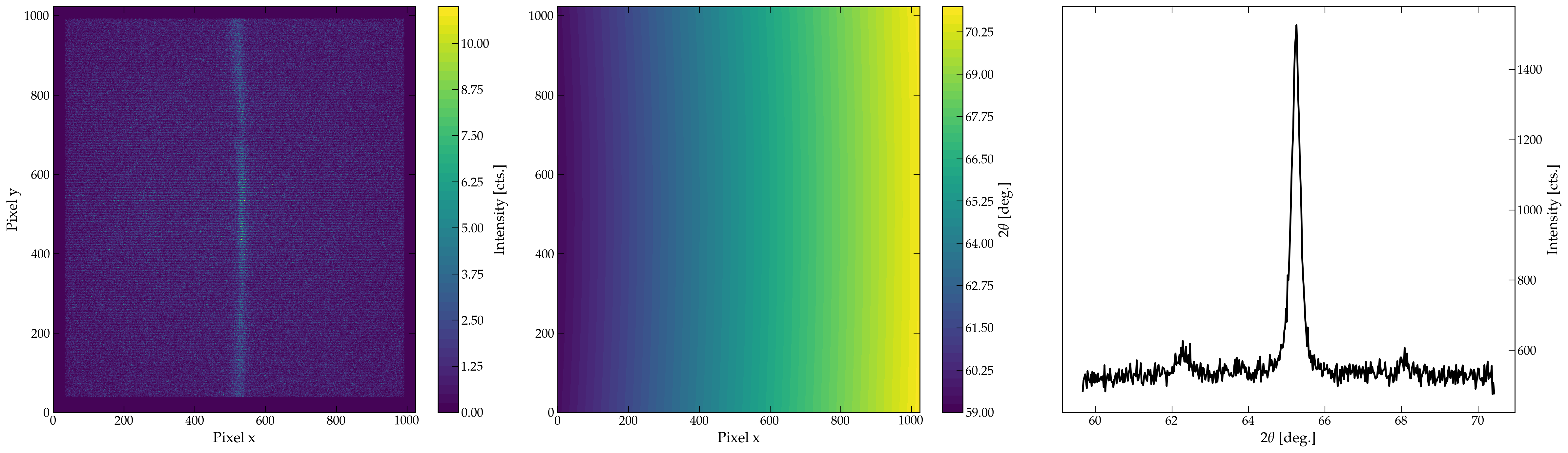
Measured data are histogrammed into a 1D diffraction dataset based on the 2θ pixel position using the numpy.histogram routine for a user-defined 2θ range and number of bins.17 We note that pyRS does not implement a sub-pixel splitting routine because measured diffraction data (1024 x 1024) represent a super-sampling of the X, Y delay lines of the DYNEX detector. A final 1D data determined by normalizing raw 1D data using vanadium dataset
Where I_N(2θ) and I(2θ)V are the histogrammed 1D patterns of the N sub-run and vanadium datasets, and T is the total time the vanadium was measured. The reduction of a representative dataset is shown in Figure 3. Normalizing each raw 1D data using a vanadium dataset provides corrections for 1) scattering angle-dependent solid angle, and 2) flat-field correction. See SFIG X for a comparison of a representative dataset before and after vanadium normalization. We note that normalization is performed after data are histogrammed into 1D to reduce the overall computational expense.
Azimuthal data reduction
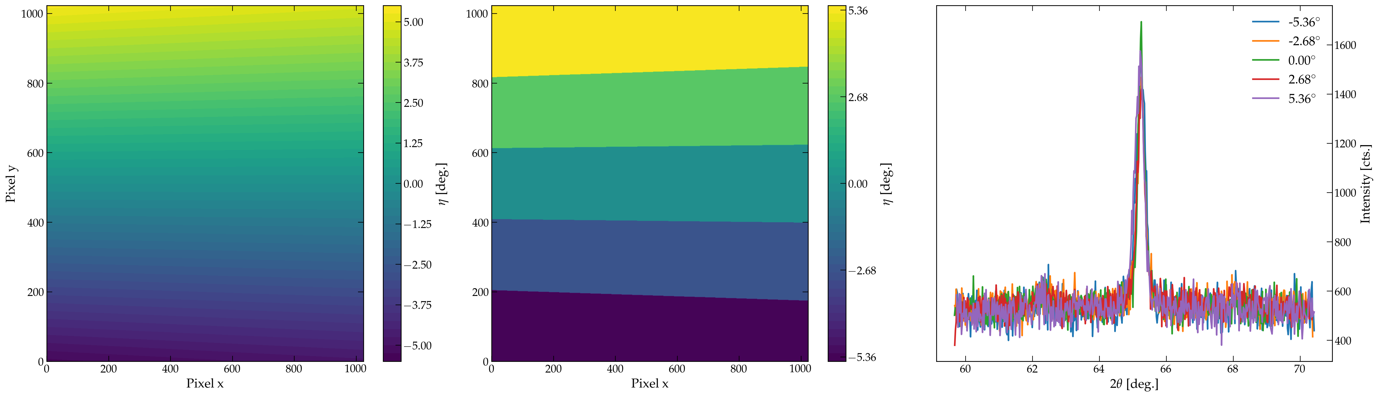
pyRS provides users the option to reduce specific regions of the 2D data into an azimuthal angle-dependent 1D dataset I(2θ, η). The implemented azimuthal integration builds upon the standard powder reduction (including vanadium normalization and error propagation) by isolating a specific η region of interest(s) (ROI) that is reduced. Users define the number of ROIs and/or minimum and maximum η. pyRS isolates the specific ROIs based using the η map constructed from (x, y, z) pixel coordinates (eq. 2). Figure 4 illustrates how specific regions from the 2D η map are isolated for reducing a representative data set into 1D I(2θ, η) data using a 2.68° azimuthal range.
Uncertainties Propagation
Uncertainties in the measured neutron events are propagated to the reduced 1D pattern using the following relation:
Where the uncertainty of each pixel takes the form of Poisson statistics.
A pixel with no count is assumed to have an uncertainty of 1.
Instrument Calibration
Diffraction Data Analysis
Strain/Stress Analysis
pyRS determines residual stresses using information about elastic strains measured for three (or two) orthogonal strain directions at concurrent spatial positions. Bragg’s law is used to determine the interatomic spacing from peak-fitting analysis of measured diffraction data.
Spatially dependent elastic strains are determined using a stress-free reference for each of the principal strain components (11, 22, and 33).
pyRS implements options for users to define a single d0 for an entire stress/strain analysis or use a spatially varying d0. A position-dependent d0 is vital for achieving an accurate representation of the strains in materials with compositional inhomogeneity (e.g., dissimilar welds) because slight differences in chemistry will change the stress-free reference. Principle residual stresses (i = 1, 2, 3) are calculated from the measured elastic strains using Young’s Modulus (E) and Poisson’s ratio (v) by
For simplicity, the spatially dependent stresses and strains are represented as σii and εii. The stress/strain UI in pyRS allows for users to impose a 2D plane stress (\(\sigma_{33}=0\)) or plane-strain (\(\epsilon_{33}=0\)) conditions. When selected, the UI only allows users to define two strain components and requires the user to define if the plane-stress or plane-strain conditions are imposed. Plane stress impacts the underlying residual stress determination because residual stresses are calculated using a simplified relationship
pyRS also calculates \(\epsilon_{33}\) for visualization purpose.
Autoreduction
The autoreduction service plays an important role in the analysis of measured data at HIDRA. By default, autoreduction converts raw neutron events into fully corrected 1-D intensity vs scattering datasets (see 2.1) immediately after measurements are completed. Autoreduction of measured data is accomplished using the pyRS scripting interface. This implementation provides access to all aspects of the pyRS framework. However, many of the underly frameworks are not enabled by default because they require user input (e.g., peak fitting analysis). The HIDRA instrument team maintains a default set of inputs that define the up-to-date calibration and vanadium inputs. Users have access to a local reduction configuration file that allows customization of inputs for the autoreduction (initialized with default parameters). Table 2 summaries the user accessible inputs for the autoreduction service. These parameters allow the users to tailor what processes are performed during the autoreduction step. Users can control how coarse or finely the measured data are binned by changing the tth_bins parameter. Defining eta_mask_angle enables the reduction of azimuthal dependent diffraction data (see 2.1.2). The peaks_file allows users to enable automated peak analysis of the measured diffraction data by specifying a json peak definition file (same format as is exported by the peakfitting UI).
[REDUCTION]
calibration_file = /HFIR/HB2B/shared/CALIBRATION/HB2B_Latest.json
vanadium_file = 2130
mask = /HFIR/HB2B/shared/CALIBRATION/MASK/HB2B_Mask_2019-11-18.xml
eta_mask_angle =
extra_logs =
tth_bins = 720
peaks_file =
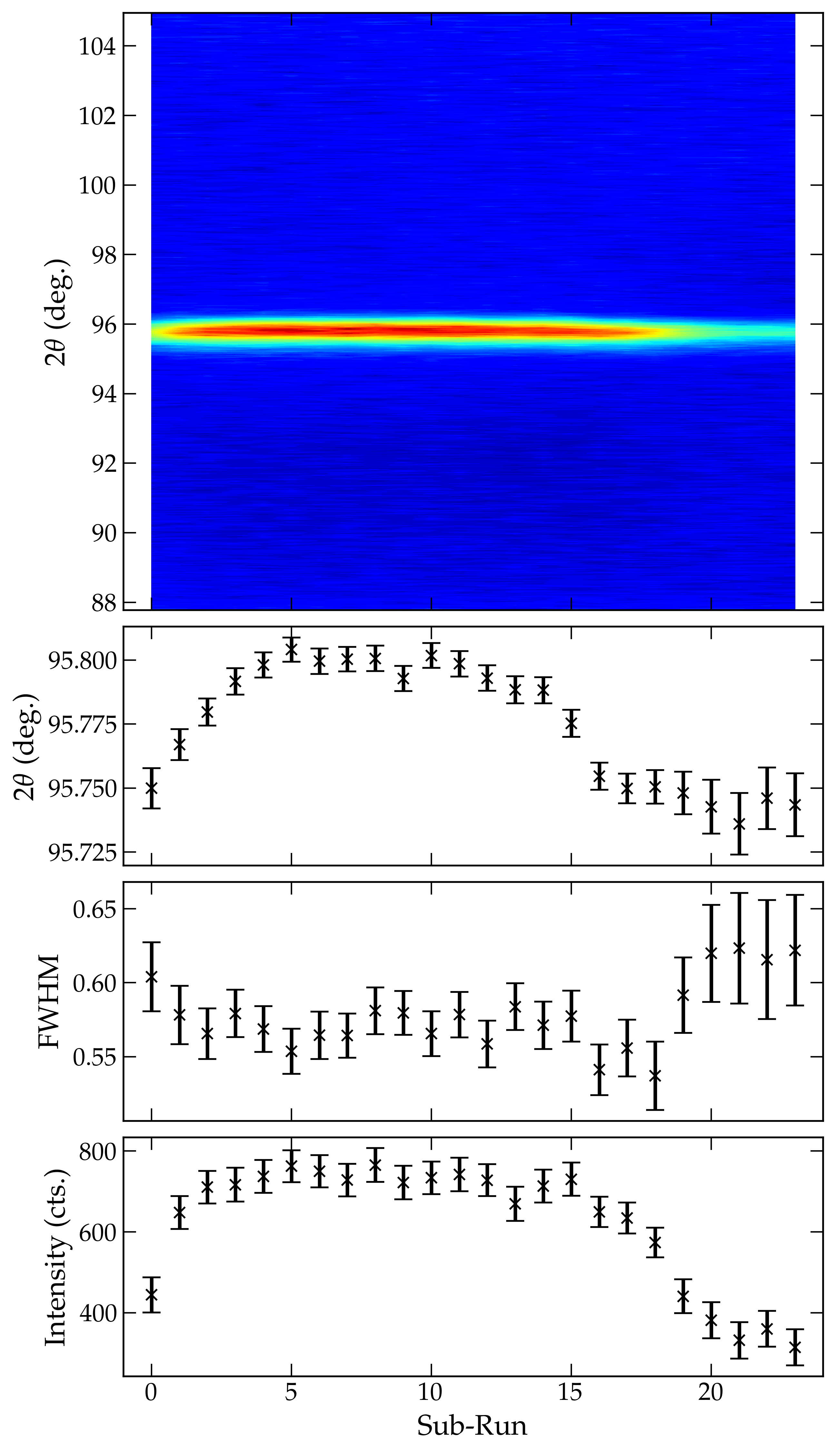
The autoreduction service provides a flexible method for both reduction and partial analysis of measured diffraction data. Results from the autoreduction are automatically published to a user-access controlled webpage for easily visualization of the results (monitor.sns.gov) using the plot.ly framework.23 Figure 8 shows representative information that is access to the users. This dataset was automatically analyzed via single peak fitting, which allows the visualization of key peak-shape parameters (peak center, FWHM, and intensity). Only a 2D contour (or 1D if only one subrun is present) of the measure diffraction data is shown if the peaks_file is undefined. We note that the plots published on monitors are for quick visualization and are not well suited for use in publications.